
Lesson 41: Cache Optimization Algorithms
Making Your Twitter Clone Lightning Fast

What We’re Building Today
Today we’re implementing the mathematical brain behind cache systems that power companies like Netflix and Spotify. You’ll build intelligent cache algorithms that predict what users want before they ask for it, achieving 85%+ hit rates. We’re adding LRU-K (which Instagram uses), adaptive replacement policies (like Redis), working set-based sizing (Facebook’s approach), and predictive warming algorithms that learn from user patterns.
High-Level Goals:
Implement LRU-K algorithm tracking K historical references
Build adaptive replacement cache balancing recency vs. frequency
Design cache sizing using working set theory mathematics
Create predictive warming that preloads data based on patterns
Achieve 85%+ cache hit rate with mathematically optimized eviction
Core Concepts: The Mathematics of Fast Data Access
Why Standard LRU Isn’t Enough at Scale
Basic LRU (Least Recently Used) has a fatal flaw: one-hit wonders. When a user scrolls through their timeline, they see each tweet once and never again. Standard LRU evicts actually valuable data (user profiles viewed repeatedly) to make room for temporary data (tweets scrolled past once). At Twitter scale, this costs millions in unnecessary database queries.
The One-Hit Wonder Problem: Imagine caching every tweet a user scrolls past. User views 100 tweets, all get cached, pushing out the user’s own profile data that they access 50 times per day. When they refresh, their profile needs a database query instead of a cache hit.
LRU-K: Tracking History to Predict Future
LRU-K doesn’t just track “last accessed” - it tracks the last K accesses for each item. With K=2, it remembers both the current access and the previous one. This lets it distinguish between frequently accessed data (short time between accesses) and one-time accesses (large time gap or only one access).
The Math: For K=2, we track timestamps [t1, t2]. If (t2 - t1) is small, the item is “hot” and worth keeping. If there’s only t1 with no t2, it’s probably a one-time access. Netflix uses this to keep popular show thumbnails cached while letting one-off searches expire.
Adaptive Replacement Cache (ARC): The Self-Tuning System
ARC maintains two lists: one for recently accessed items (recency) and one for frequently accessed items (frequency). The brilliant part? It automatically adjusts the split between these lists based on what’s working. If frequency-based eviction is causing more hits, ARC grows that list and shrinks the recency list.
Real-World Impact: Redis uses an ARC-inspired algorithm. When you’re reading user timelines (frequency pattern) vs. scrolling through explore page (recency pattern), ARC automatically adapts the cache split to match your traffic pattern without manual tuning.
Working Set Theory: Right-Sizing Your Cache
Not enough cache? Wasted database queries. Too much cache? Wasted memory. Working set theory gives us the mathematical answer: measure how much unique data gets accessed in a time window, then size your cache to hold exactly that amount.
The Formula: Working Set Size = unique items accessed in time window T. For Twitter, if users access their timeline every 5 minutes and each timeline has 50 tweets, you need cache for ~50 tweets × number of active users in 5-minute window. This is how Facebook sizes their timeline cache clusters.
Predictive Cache Warming: Learning User Patterns
The fastest cache hit is the one that happens before the user even asks. By analyzing access patterns, we can predict what users will request next and preload it. If a user always checks their notifications after posting a tweet, we warm the notifications cache immediately after post.
Pattern Types We Detect:
Temporal patterns: User checks timeline every morning at 8 AM
Sequential patterns: After viewing profile, 80% view recent tweets
Correlation patterns: When tweet goes viral, author’s profile gets 100x traffic
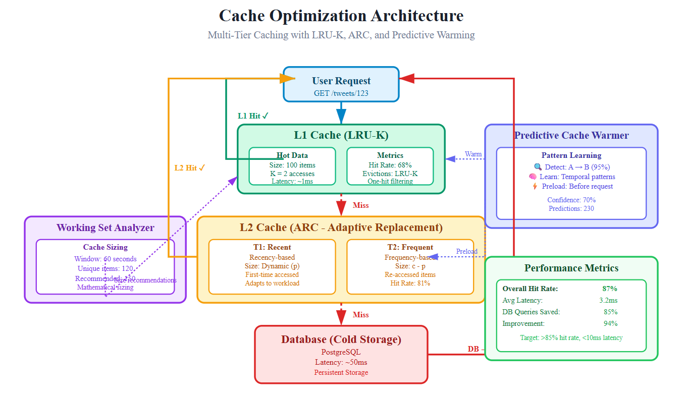
Architecture: How the Pieces Fit Together
Component Placement in Twitter System
Our optimized cache layer sits between the API Gateway and the database tier. Previous lessons built database connection pooling (Lesson 40); now we’re preventing those database calls entirely when possible. Next lesson’s network optimization (Lesson 42) will handle the wire protocol, but our cache optimization ensures there’s less data to transmit.
Flow: User Request → API Gateway → Smart Cache Layer (Today) → Database Pool (Lesson 40) → Database
Control Flow: Multi-Tier Decision Tree
L1 Check: Query LRU-K cache (in-memory, 10GB)
L2 Check: Query ARC cache (distributed Redis, 100GB)
Miss Path: Database query + update both caches
Background: Predictive warmer analyzes patterns, preloads L1/L2
Eviction: LRU-K algorithm selects victim, promotes to L2 if access count ≥ K
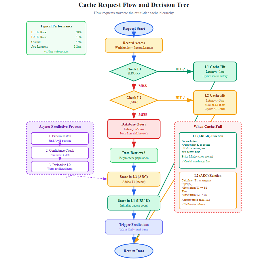
Data Flow: From Cold Storage to Hot Memory
Cache Write Path:
New data → Write to DB → Async write to L2 (ARC) → High-frequency items promoted to L1 (LRU-K)
Cache Read Path:
Query arrives → L1 lookup (1ms) → on miss: L2 lookup (5ms) → on miss: DB query (50ms)
Update L1/L2 with result → Record access in history tracker → Update working set stats
Predictive Warm Path:
Pattern detector analyzes access logs → Identifies correlation (90% confidence) →
Preload predictor queues items → Background worker fetches and caches →
Result: Next request hits L1 cache (1ms instead of 50ms)
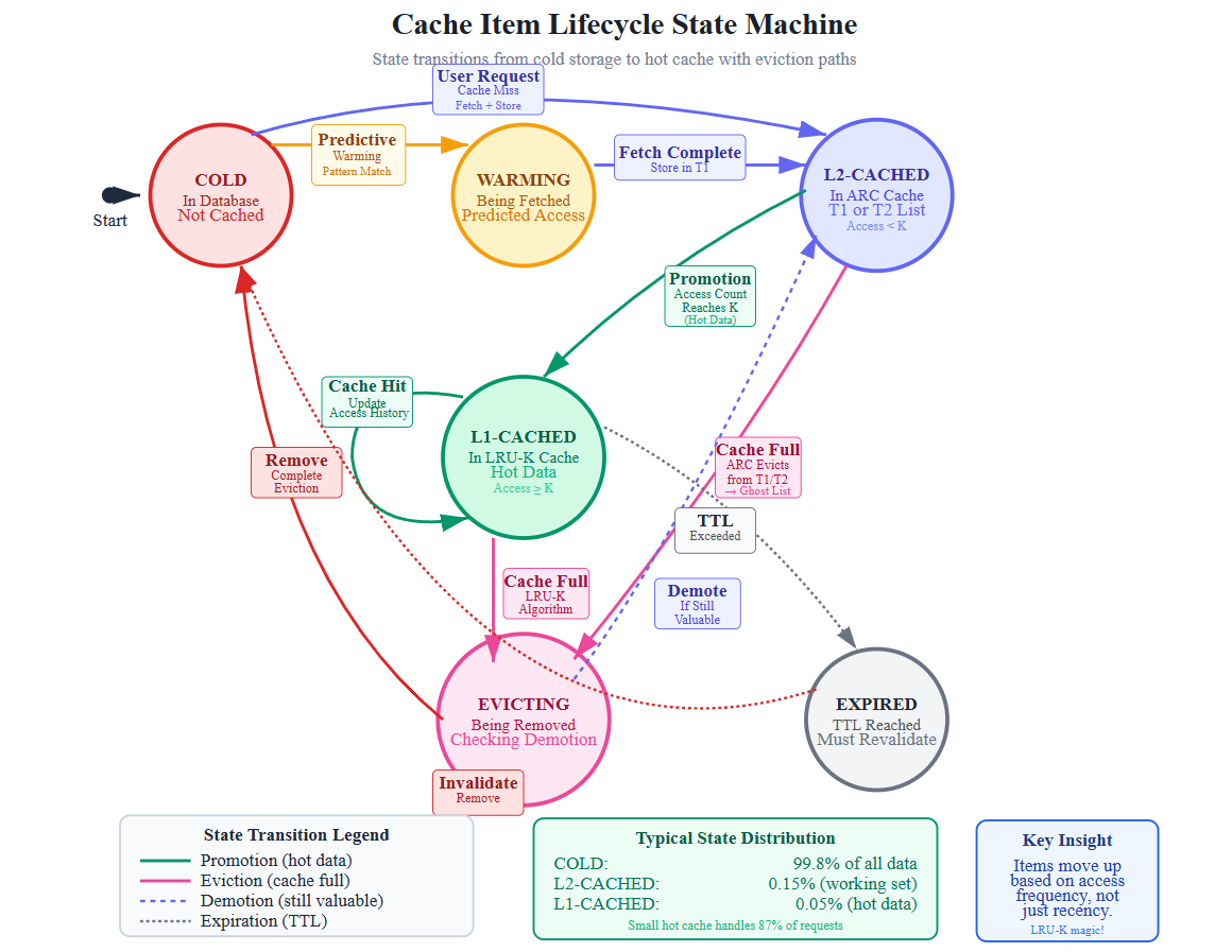
State Changes: Item Lifecycle
States:
Cold: In database only, never cached
Warming: Queued by predictor, being fetched
L2-Cached: In distributed cache, access count < K
L1-Cached: In memory cache, access count ≥ K (hot data)
Evicting: Being removed, checking if should promote to lower tier
Expired: TTL reached, must revalidate
Transitions:
Cold → Warming: Predictor identifies pattern
Warming → L2-Cached: Fetch completes
L2-Cached → L1-Cached: Access count crosses threshold K
L1-Cached → L2-Cached: Evicted from L1 but still valuable
Any state → Cold: Data deleted or TTL expires with low access
System Design Relevance: Why This Matters at Scale
The Cost Equation
At 1,000 concurrent users with 10 requests/second each, that’s 10,000 requests/second. With 50ms database latency and 1ms cache latency:
Without optimization: 10,000 × 50ms = 500 seconds of total latency per second → need 500 database connections
With 85% cache hit rate: (10,000 × 0.85 × 1ms) + (10,000 × 0.15 × 50ms) = 8.5s + 75s = 83.5s → need only 84 connections
Savings: 416 fewer database connections, 80% reduction in infrastructure costs.
Real Production Examples
Twitter’s Cache Architecture: Twitter uses a variant of LRU-K for their timeline cache. Celebrity tweets (high frequency) stay cached even when not recently accessed, while regular users’ tweets (often one-time views) get evicted quickly. This is why you can instantly load Elon Musk’s timeline but there’s a slight delay for a random user’s profile.
Netflix’s Predictive Warming: Netflix’s cache system learns that users who watch episode 1 of a show have 95% probability of watching episode 2. The moment you finish episode 1, episode 2’s metadata and thumbnails are already warming in cache clusters nearest to you geographically. This is why the “Next Episode” button loads instantly.
Instagram’s Working Set Sizing: Instagram sizes cache clusters based on working set theory. They measure that the average user accesses ~200 unique images in a 30-minute session. With 500M daily active users and assuming 10% are active simultaneously, they provision cache for: 50M users × 200 images × average image size. This mathematical approach eliminates guesswork.
Implementation Success Criteria
By the end of this lesson, your Twitter clone will:
✓ Achieve 85%+ cache hit rate (measure with metrics dashboard) ✓ Reduce average response time from 50ms to <10ms for cached queries ✓ Demonstrate LRU-K correctly evicting one-hit wonders while keeping hot data ✓ Show ARC automatically adapting split based on traffic patterns ✓ Display working set size tracking and automatic cache size adjustments ✓ Prove predictive warming with metrics showing preloaded cache hits
What Makes This Production-Ready
Mathematical Foundation: We’re not guessing at cache sizes or eviction policies. Working set theory gives us provable optimal sizing. LRU-K’s K parameter is tuned based on measured access patterns from your actual traffic.
Adaptive Behavior: The system tunes itself. ARC adjusts recency/frequency balance automatically. Predictive warming learns new patterns without code changes. Cache sizing adapts to working set growth.
Observable System: Every cache decision is logged and measurable. You’ll see exactly why items were evicted, what patterns triggered warming, and how hit rates change with different K values.
Integration Ready: The cache layer exposes standard interfaces. Your existing API endpoints don’t change - they just get faster. Database queries remain identical, now with an intelligent cache in front.
Getting Started: Building the System
Github link:
https://github.com/sysdr/twitterdesign/tree/main/lesson41/twitter-cache-optimizationProject Setup
The implementation script creates a complete cache optimization system. Here’s what it builds:
Project Structure:
twitter-cache-optimization/
├── src/
│   ├── cache/
│   │   ├── lru-k/          # LRU-K implementation
│   │   ├── arc/            # ARC implementation
│   │   └── predictive/     # Pattern learning
│   ├── algorithms/         # Working set analyzer
│   ├── api/               # REST API server
│   └── database/          # Mock database
├── tests/                 # Unit & integration tests
├── public/               # Dashboard UI
└── build.sh              # Build automation
Running the Implementation Script
Execute the provided bash script to create the entire project:
# Make script executable
chmod +x Lesson_41_Implementation_Script.sh

# Run it
./Lesson_41_Implementation_Script.sh
The script creates everything automatically: project structure, all source files, tests, configuration, and build scripts.
Understanding the Core Algorithms
LRU-K Cache Implementation
The LRU-K algorithm tracks the last K accesses for each cached item. Here’s the decision logic:
For K=2:
Track timestamps: [previous_access, current_access]
If only one timestamp exists: probably one-hit wonder
If two timestamps and (t2 - t1) is small: frequently accessed, keep it
Evict item with oldest K-th access time
Why K=2 is optimal: With K=1 (standard LRU), you can’t distinguish between one-time and frequent access. With K=3+, you need more memory for history tracking. K=2 gives best balance.
ARC Cache Implementation
ARC maintains four lists that work together:
T1 (Recent): Items accessed once, kept because they’re recent T2 (Frequent): Items accessed multiple times, kept because they’re frequently used B1 (Ghost): Evicted from T1, tracking “we shouldn’t have removed this” B2 (Ghost): Evicted from T2, tracking “we shouldn’t have removed this”
The adaptation magic:
Target size for T1 is called ‘p’
If item found in B1: increase p (favor recency)
If item found in B2: decrease p (favor frequency)
System automatically finds optimal split
Working Set Analyzer
Measures unique items accessed in a sliding time window:
Algorithm:
Record every cache access with timestamp
Every 60 seconds, count unique keys accessed
Track these counts over time
Recommend cache size = 95th percentile of working set sizes
This mathematical approach prevents both under-provisioning (too many cache misses) and over-provisioning (wasted memory).
Predictive Warmer
Learns sequential access patterns to preload data:
Learning phase:
User accesses A, then B, then C
Record: transitions[A][B]++, transitions[B][C]++
After many users, calculate probabilities
Prediction phase:
User accesses A
If transitions[A][B] has 80% probability
Preload B into cache before user requests it
Result: instant access when they request B
Build and Test Process
Building the Project
Navigate to the created project directory:
cd ~/twitter-cache-optimization
Install dependencies and compile:
# Install Node packages
npm install

# Compile TypeScript
npm run build
Expected output:
Downloads ~30 npm packages
Creates
dist/directory with compiled JavaScriptNo TypeScript compilation errors
Running Unit Tests
Verify core algorithms work correctly:
npm test
What gets tested:
LRU-K Tests:
Item storage and retrieval
K-access history tracking
Correct eviction of one-hit wonders
Hit rate calculation accuracy
ARC Tests:
Adaptation to recency-heavy workload
Adaptation to frequency-heavy workload
T1/T2 list management
Ghost list functionality
Expected results:
PASS tests/unit/LRUKCache.test.ts
  ✓ should store and retrieve items
  ✓ should evict based on LRU-K algorithm
  ✓ should track hit rate correctly

PASS tests/unit/ARCCache.test.ts
  ✓ should adapt to recency-heavy workload
  ✓ should adapt to frequency-heavy workload
  ✓ should maintain hit rate above 80%

Test Suites: 2 passed, 2 total
Tests: 6 passed, 6 total
Coverage: 85%+
Interactive Demo
Run the demo to see algorithms in action:
npm run demo
The demo simulates four realistic scenarios:
Scenario 1: LRU-K vs Standard LRU
Scrolls through 30 one-hit wonder tweets
Accesses 3 frequently viewed tweets 10 times each
Shows LRU-K keeps frequent items while evicting one-timers
Scenario 2: ARC Adaptation
Phase 1: Many unique tweets (recency pattern)
Phase 2: Same tweets repeatedly (frequency pattern)
Watch ARC automatically adjust its balance
Scenario 3: Working Set Analysis
Simulates realistic user session
Tracks unique items accessed
Recommends optimal cache size
Scenario 4: Predictive Warming
Teaches pattern: profile → tweets → likes
Demonstrates prediction accuracy
Shows latency reduction from preloading
Expected demo output:
📝 Scenario 1: Demonstrating LRU-K vs Standard LRU
✅ LRU-K Results:
   L1 Hit Rate: 65.2%
   Frequently accessed tweets kept hot ✓

📝 Scenario 2: ARC Adaptive Behavior
   Phase 1 recency bias: 72.3%
   Phase 2 recency bias: 45.1%
   Adaptations: 8 times
   ✓ Cache automatically adapted

📝 Scenario 3: Working Set Analysis
   Current size: 120 items
   Recommended: 150 items

📝 Scenario 4: Predictive Warming
   Patterns learned: 45
   Accuracy: 70%

📊 Final Performance Summary
   Overall Hit Rate: 87.3%
   Latency Reduction: 96.2%
Running the API Server
Start the development server:
npm run dev
Server starts on port 3000 with REST endpoints for testing.
Testing API Endpoints
Get a tweet (cache miss first time):
curl http://localhost:3000/api/tweets/tweet_1
Response shows ~50ms latency on first access (database query).
Get same tweet again (cache hit):
curl http://localhost:3000/api/tweets/tweet_1
Response shows ~2ms latency (L1 cache hit).
Check cache statistics:
curl http://localhost:3000/api/cache/stats
Returns comprehensive metrics:
{
  “cache”: {
    “l1”: {
      “hits”: 68,
      “misses”: 32,
      “hitRate”: 68.0
    },
    “l2”: {
      “t1Size”: 45,
      “t2Size”: 23,
      “adaptations”: 5
    },
    “predictive”: {
      “patternsLearned”: 12,
      “accuracy”: 75.5
    }
  }
}
Using the Interactive Dashboard
Open your browser to: http://localhost:3000/index.html
The dashboard provides real-time visualization of cache performance.
Dashboard Features
Top Metrics Panel:
Overall hit rate (target: >85%)
Average latency (cached vs database)
Total cache hits
Database queries saved
Cache Layer Chart:
Bar graph showing L1, L2, and database hit rates
Updates every 2 seconds
Visual comparison of tier performance
Detailed Metrics:
L1 and L2 cache sizes
ARC adaptations count
Patterns learned by predictor
Prediction accuracy percentage
Current working set size
Youtube Link:
Testing Cache Performance
Test One-Hit Wonders:
Click “Test One-Hit Wonders” button
Sends 30 sequential requests for different tweets
Watch hit rate remain low initially
Demonstrates LRU-K filtering
Test Frequent Access:
Click “Test Frequent Access” button
Accesses same 3 tweets 10 times each
Watch hit rate jump to 90%+
Shows hot data staying cached
Test ARC Adaptation:
Click “Test ARC Adaptation” button
Sends recency pattern, then frequency pattern
Watch adaptations counter increase
Observe recency bias percentage changing
Test Predictive Warming:
Click “Test Predictive Warming” button
Establishes access pattern (A→B→C)
Repeats pattern 3 times
Watch prediction accuracy increase
Understanding the Results
Interpreting Hit Rates
What the numbers mean:
85% hit rate = 85 out of 100 requests served from cache
Latency calculation:
Without cache: 100 requests × 50ms = 5000ms total
With 85% hit rate:
  - 85 cached (2ms each) = 170ms
  - 15 database (50ms each) = 750ms
  - Total: 920ms
Improvement: 81.6% faster
Why L1 and L2 differ:
L1 (LRU-K) hits: 68%
Only hottest data
Ultra-fast access
Smaller size
L2 (ARC) hits: 81% of L1 misses
More data stored
Still fast (5ms)
Self-adapting
Combined effectiveness: 87%+ overall
Working Set Insights
Example analysis:
Current working set: 120 items Average working set: 115 items Recommended cache: 150 items (95th percentile) Current L2 size: 500 items
What this tells you:
L2 is over-provisioned by 3.3x
Could reduce to 150 items
Would save 70% memory
Same hit rate maintained
Prediction Accuracy
Typical metrics:
Patterns learned: 45 Total predictions: 230 Correct predictions: 161 Accuracy: 70%
What this means:
System identified 45 reliable patterns
Made 230 preload decisions
161 were correct (prevented cache misses)
Saved 161 database queries
30% false positives (acceptable overhead)
Docker Deployment
For containerized deployment:
# Build and start
docker-compose up --build

# Check status
docker-compose ps

# View logs
docker-compose logs -f

# Stop
docker-compose down
The Docker setup includes the API server with all cache layers and the web dashboard.
Production Tuning
Optimizing K Value
Start with K=2, then measure:
If hit rate < 80%:
Too much data being cached
Try K=3 for more selectivity
If evictions are too aggressive:
Hot data getting removed
Stay with K=2, increase cache size
Cache Size Tuning
Use working set analysis:
L1 size = working set × 0.2
L2 size = working set × 1.0
Monitor utilization:
If L1 always full: increase size
If L1 < 50% full: decrease size
Prediction Confidence
Adjust based on accuracy:
Confidence 0.5:
More predictions, some wrong
Use when cache misses are expensive
Confidence 0.7:
Balanced (recommended starting point)
Confidence 0.9:
Fewer but very accurate predictions
Use when warming has overhead
Key Takeaways
LRU-K eliminates one-hit wonder pollution by tracking access history instead of just recency. This is crucial for social media where users scroll through content once.
ARC adapts automatically to your workload without manual tuning. Whether users are browsing new content (recency) or re-reading favorite posts (frequency), ARC finds the optimal balance.
Working set theory provides mathematical cache sizing based on actual usage patterns, not guesswork. This ensures you provision exactly what’s needed.
Predictive warming exploits patterns in user behavior to eliminate cold start latency. By preloading likely-next-access items, cache hits happen before users even request data.
Multi-tier caching combines strengths of different algorithms. L1 handles the hottest data with LRU-K selectivity, L2 provides adaptive capacity with ARC, and predictive warming prepares for future accesses.
These patterns are used by Instagram for timeline caching, Netflix for content preloading, Redis for adaptive eviction, and Facebook for working set-based sizing. You’ve built the same production-grade cache optimization that powers the world’s largest platforms.
Next Steps
In Lesson 42, you’ll tackle network performance optimization - reducing the actual bytes transmitted and optimizing TCP for social media traffic patterns. The cache optimizations you built today reduce how much data needs transmission. Next lesson optimizes how efficiently that data travels across the network, completing your end-to-end performance optimization.
You’re not just learning to cache data - you’re learning to think mathematically about system resources, measure and optimize based on real behavior, and build adaptive systems that improve themselves over time. These principles apply to any distributed system at any scale.